Laptop Price Prediction Using Random Forest Regressor with MLflow
In the world of machine learning, managing experiments, tracking models, and sharing results are crucial aspects of any successful project. MLflow has emerged as a powerful tool for experiment tracking and model management, simplifying these processes and ensuring reproducibility. In this blog, I’ll guide you through the steps of integrating MLflow into your machine learning workflow, from setting up an MLflow server and tracking experiments, to packaging your code as an MLflow project. Whether you’re collaborating with a team or working solo, MLflow makes it easier to track your work and share results.
Let’s dive into how you can streamline your ML process and make your experiments more manageable and reproducible.

“MLOps is the bridge between machine learning and production, ensuring that models are not just built, but continuously delivered, maintained, and improved.”
1. Exploring the Laptop Dataset: A Data Science Journey
As data scientists, our journey often starts with understanding the dataset at hand. For this project, I worked with a dataset containing various attributes of laptops, gathered from an e-commerce platform. The goal was to predict the price of laptops based on features such as brand, RAM size, storage, ratings, and more.

Here’s an overview of the original columns in the laptop dataset:
- Laptop Name: The name of the laptop (e.g., “HP Spectre x360”). This column didn’t contribute to price prediction, so it was dropped during data cleaning.
- Link: URL links to the product. Irrelevant for price prediction, so it was removed.
- Seller Name: The name of the seller, which doesn’t provide any insight into the laptop’s price and was discarded.
- Door Delivery Fees & Pickup Fees: Although these could impact the total cost to the customer, they don’t influence the base price of the laptop, so they were removed.
- Old Price and Current Price: Both of these columns were redundant because we already had the standardized USD Price column, which we used for price prediction.
- Rating_out_of_5 and Number of Ratings: These two columns are highly correlated — higher ratings usually come with more reviews. Instead of using them separately, we combined them into a new feature called Weighted Reviews to capture both the quality and volume of feedback.
- ROM (Storage): Contained values like “512GB SSD” or “1TB HDD”, which were difficult to use directly in machine learning models. This was split into two separate columns: Storage (size only, e.g., “512GB”) and isSSD (a binary indicator of whether the laptop uses an SSD).
- Sale Type: Indicates whether the sale is from an official store or verified store, which is a categorical variable.
- Brand: The brand of the laptop, which is another categorical feature.
- RAM: The size of the RAM, an important numeric feature influencing the price.
- Seller Score: This column had some missing values that we needed to handle.
With this initial exploration in mind, we can move forward with data cleaning and feature engineering.
2. Exploratory Data Analysis (EDA): Unveiling Insights from the Data
Before we jump into any machine learning model, it’s important to explore the data and uncover hidden patterns. Exploratory Data Analysis (EDA) is like a treasure hunt for data scientists. Here’s how I approached it:
Data Distribution:
The first thing I looked at was the distribution of the target variable (price). A quick look at the histogram revealed that the prices were skewed, meaning we might need to perform some transformations to make the data more manageable.
Missing Values:
Missing values can be a challenge in any dataset. For instance, some features like ‘Seller Score’ were missing data, which could negatively impact model training. I used the median to fill in these gaps, as it ensures that our data remains representative without distorting the overall trends.
Outliers:
Outliers are extreme values that can mess with our model’s predictions. By using box plots and scatter plots, I identified some outliers in features like RAM and Storage, which were cleaned up accordingly.
Feature Relationships:
One of the coolest parts of EDA is discovering relationships between variables. For example, I found that higher RAM and bigger storage were strongly correlated with higher prices. This is important because it helped me understand what factors influence price the most.
Through this process, I not only got familiar with the dataset but also identified potential features that might impact our model’s predictions. Let’s see how we cleaned and transformed the data in the next step!
3. Data Cleaning and Feature Engineering: Preparing the Data for Machine Learning
With the insights from EDA in hand, it was time to clean the data and engineer new features to enhance model performance. Here’s a look at what I did:
Dropping Irrelevant Columns
Several columns that didn’t contribute directly to the target variable (laptop price) were removed:
- Laptop Name, Link, and Seller Name were discarded as they weren’t useful for price prediction.
- Door Delivery Fees and Pickup Fees were removed, as these are related to total cost rather than the laptop’s base price.
Consolidating Price Information
- The dataset included both Old Price and Current Price columns. Since we had the more standardized USD Price, both were dropped to avoid redundancy and to maintain consistency across the dataset.
Combining Rating Information
- The Rating_out_of_5 and Number of Ratings columns were merged into a new feature: Weighted Reviews, which combines both the quality and the volume of customer feedback. This proved to be a better predictor for price estimation than the original columns.
Handling Storage (ROM) Information
- The ROM column contained storage information in a mixed format like “512GB SSD” or “1TB HDD,” which was not directly usable. So, we split this column into two new features:
- Storage: This column now contains just the storage size (e.g., “512GB”, “1TB”).
- isSSD: A binary feature indicating whether the laptop uses an SSD (1 for SSD, 0 for HDD).
This transformation made it easier for the model to process and understand the data.
Encoding Categorical Features
- Columns like Sale Type and Brand are categorical. These needed to be converted into numerical features using One-Hot Encoding, which creates binary features for each category (e.g., a separate column for each brand).
Dealing with Missing Values
- Two columns had missing values:
- RAM: Missing values were imputed with the median value.
- Seller Score: Missing values were also imputed with the median, providing a reliable estimate without distorting the data distribution.
Scaling the Data:
Lastly, some features like RAM and Storage had vastly different scales, which could affect model performance. I applied MinMaxScaler to normalize the data, ensuring all features are on the same scale.
After these transformations, the data was finally ready for model training! But before jumping into machine learning, I needed to evaluate the performance of different algorithms. That’s coming up next.
4. Exploring Different Models: Finding the Best Fit for Our Data
Now that our data was clean and ready, it was time to dive into the exciting world of machine learning models. The goal was to find the best model to predict the laptop prices. Here are the models I experimented with:
Linear Regression (LR):
I started with a simple Linear Regression model. It gave a decent baseline, but since the relationships between features and price aren’t purely linear, I knew I had to try more complex models.
K-Nearest Neighbors (KNN):
KNN is a simple yet powerful model. It calculates the average price of the K-nearest data points to make predictions. While it did okay, it struggled with the scaling of features and required careful tuning.
Random Forest Regressor (RF):
Next, I tried Random Forest Regressor — a more powerful model that can handle non-linear relationships. It’s great at capturing interactions between features without overfitting. This model showed promising results and was able to handle both categorical and continuous features effectively.
XGBoost Regressor:
XGBoost is one of the most popular models for structured data. I gave it a try, and it performed well. It’s a boosting algorithm that builds trees sequentially, making it very accurate for complex datasets like this one.
Elastic Net Regressor:
Finally, I tested Elastic Net, which combines the strengths of both Lasso and Ridge regression. This model is useful when there’s multicollinearity (high correlation between independent variables). It helped me see if regularization could improve performance.
After experimenting with different models, Random Forest Regressor emerged as the clear winner, delivering the best performance in terms of both Mean Absolute Error (MAE) and R-squared (R²).
5. Integrating MLflow for Reproducibility:
To streamline the process of tracking experiments, serving models, and making predictions, we integrate MLflow into the workflow. This integration allows for efficient experiment management, model deployment, and inference. Below are the steps involved in setting up and using MLflow within the project.

5.1 Setting Up MLflow Server
To expose your model through MLflow, we start by setting up an MLflow server in a Docker container. This provides a centralized place to track experiments and serve models. Follow these steps to configure the MLflow server:
- Create a Dockerfile for MLflow: In the
mlflow-serverfolder, create aDockerfileto build a Docker image for the MLflow server:
FROM python:3.7-slim-stretch

# Install mlflow
RUN python -m pip install --upgrade pip mlflow==1.4.0

# Expose mlflow port
EXPOSE 1234

# Define entry point
ENTRYPOINT mlflow server --host 0.0.0.0 --port 1234- Create a
docker-compose.yamlFile: In the root folder, create adocker-compose.yamlfile to build and start the MLflow server:
version: '3.1'

services:

  mlflow-server:

    build:

      context: ./mlflow-server
        dockerfile: Dockerfile

    image: mlflow:1.4.0

ports: - "1234:1234"- Start the MLflow Server: Use Docker Compose to build and run the MLflow server by executing the following command:
docker-compose up --build mlflow-server- Set Up Environment Variables: Create a
.envfile in the root directory with the following content to configure the MLflow tracking URI:
MLFLOW_TRACKING_URI=http://localhost:1234- Launch the MLflow UI: Start the MLflow UI to monitor experiments by running the command:
mlflow ui --host 127.0.0.1 --port 1234
5.2 Tracking Experiments in MLflow
To track experiments, log the model and its parameters during training. In the train.py script, use the following function to get or create an MLflow experiment:
from mlflow import MlflowClient
from mlflow.entities import Experiment, RunInfo
import mlflow
import logging

logger = logging.getLogger(__name__)
def get_or_create_experiment(experiment_name) -> Experiment:
    """
    Creates an MLflow experiment if it doesn't already exist.
    """
    try:
        client = MlflowClient()
        experiment = client.get_experiment_by_name(name=experiment_name)
        if experiment and experiment.lifecycle_stage != 'deleted':
            return experiment
        else:
            experiment_id = client.create_experiment(name=experiment_name)
            return client.get_experiment(experiment_id=experiment_id)
    except Exception as e:
        logger.error(f'Unable to get or create experiment {experiment_name}: {e}')
Next, use the function log_metrics_and_model to log model parameters and metrics to MLflow:
def log_metrics_and_model(pipeline, test_metric_name: str, test_metric_value: float):
    experiment_name = 'pulsar_stars_training'
    experiment = get_or_create_experiment(experiment_name)
    model = pipeline.steps[1][1]  # Extract the model
    best_params = model.best_params_

def build_local_model_path(relative_artifacts_uri: str, model_name: str):
        import os
        absolute_artifacts_uri = relative_artifacts_uri.replace('./', f'{os.getcwd()}/')
        return os.path.join(absolute_artifacts_uri, model_name)
    with mlflow.start_run(experiment_id=experiment.experiment_id, run_name='training') as run:
        model_name = 'sklearn_logistic_regression'
        run_info = run.info
        mlflow.log_params(best_params)
        mlflow.log_metric(test_metric_name, test_metric_value)
        mlflow.sklearn.log_model(pipeline, model_name)
        model_path = build_local_model_path(run_info.artifact_uri, model_name)
        logger.info(f'Model for run_id {run_info.run_id} exported at {model_path}')
5.3 Exposing the Model for Inference
After training and logging the model, we need to expose it for inference. Follow these steps to serve the model and make predictions:
- Add Model Path to
.env: In your.envfile, add theMODEL_PATHvariable, which stores the location of the trained model. This path will be printed at the end of the training script:
MODEL_PATH=path_to_your_model- Serve the Model Using MLflow: Run the following command to serve the model using MLflow’s model serving feature:
mlflow models serve -m ${MODEL_PATH} -p 4321- This starts a REST API server that listens on port
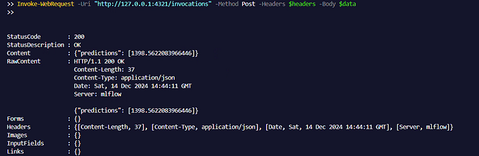
4321for inference requests. - Send Inference Requests: Use PowerShell to send a POST request to the MLflow model server with the data in the required format:
$headers = @{     "Content-Type" = "application/json" }
$data = '{     "dataframe_split": {         "columns": [
 "Discount Percentages", "Unit Available","RAM","Seller Score",
"Weighted_Rating", "Storage","isSSD", "Sale Type_Official Store",
 "Sale Type_Verified by JUMIA","Brand_Apple","Brand_Asus",
"Brand_DELL","Brand_Fujitsu","Brand_HP","Brand_Huawei",
 "Brand_ITX","Brand_Lenovo", "Brand_MSI"
],
"data": [             [140.5625, 55.68378214, -0.23457141, -0.6996484, 3.19983278, 19.11042633, 7.97553179, 74.24222492, 15, 10, 8, 4.5, 4.2, 500, 1, 1, 0, 1, 0, 0, 0, 0, 1, 0, 0, 0, 0]         ]     } }'
Invoke-WebRequest -Uri "http://127.0.0.1:4321/invocations"
-Method Post -Headers $headers -Body $data
This will send the data to the MLflow server and return the model’s prediction.
Creating the Conda Environment with conda.yaml
In this section, we’ll walk through how to package our training code as an MLflow project, making it reproducible and easier to share. This process allows you to run the code from any environment using a single command, and it ensures that all dependencies and configurations are tracked.
The first step in packaging your code as an MLflow project is to define the environment where the code will run. This is done by creating a conda.yaml file, which lists all the necessary dependencies.
Here’s what a basic conda.yaml might look like for our project:
name: mlflow-env

channels:
  - defaults

dependencies:
  - python=3.7.3
  - pip:
    - scikit-learn==0.21.3
    - mlflow
    - cloudpickle==1.2.2
    - google-cloud-storage
    - python-dotenv
    - pandas
This file specifies the Python version and includes important libraries like scikit-learn, pandas, and mlflow. Once you have this file, you can use it to set up the environment in any machine where the project will run.
5.2 Defining the MLflow Project with MLproject
Now, let’s make our project executable using the mlflow run command. This is done by creating an MLproject file that tells MLflow how to run the code and which parameters to pass.
Here’s an example of how to set up the MLproject file:
name: mlflow-laptop-estimator  #chose your project name

conda_env: {your folder}/conda.yaml  #change the placeholder by your folder that contain train.py

entry_points:
  main:
    parameters:
      data_path: string
      test_size: {type: float, default: 0.2}
    command: "python psp/training.py --data-path {data_path} --test-size {test_size}"
The MLproject file specifies that we want to use the conda.yaml environment for dependencies and defines the main script to execute. We’re passing in two parameters: data_path and test_size. The command section defines how the training script will be executed with these parameters.
5.3 Setting Up Remote MLflow Tracking Server
In our case, we are using a remote MLflow tracking server hosted on Google Cloud. This means we don’t need to set up a local server but instead will be communicating with a server hosted on a Google Compute Engine instance.
Before running the project, you’ll need to configure the environment variables so that MLflow knows where to send the data:
export MLFLOW_TRACKING_URI=http://34.89.15.138
export MLFLOW_TRACKING_USERNAME="ms-bgd"
export MLFLOW_TRACKING_PASSWORD="xxx"  # This password will be shared
These environment variables ensure that MLflow knows where to send tracking information, such as metrics and model artifacts, as well as how to authenticate with the server.
5.4 Running the MLflow Project
With everything set up, you can now run your training code using the MLflow command line interface. This makes it easier to execute the same script across different environments and ensures consistency in the results.
mlflow run . -P data_path=./data/pulsar_stars.csvThis command runs the project in the current directory and passes the data_path as a parameter to the script. MLflow will log all metrics, parameters, and model artifacts to the remote tracking server.
5.5 Verifying Reproducibility
One of the key benefits of using MLflow is that it makes your work reproducible. This means that anyone, anywhere, with access to the right environment can run your project and get the same results.
To verify this, you can try running the project on another machine or from a different location. Here’s how:
- Set the data path on your new machine:
export DATA_PATH=xxx cp ./data/pulsar_stars.csv $DATA_PATH- Run the project from GitHub:
mlflow run git@github.com:ngallot/mlflow-demo.git -P data_path=${DATA_PATH}By running the project from GitHub, you can confirm that the MLflow project is fully reproducible, as the exact same results will be obtained no matter where the code is executed.
5.6 Next Steps: Improving the Model
Now that your code is reproducible and tracked by MLflow, you can focus on improving the machine learning model. MLflow makes it easy to iterate on models, tweak hyperparameters, and keep track of all versions of the model.
Conclusion:
By integrating MLflow into your machine learning pipeline, you gain valuable insights into your model’s performance, track the evolution of your experiments, and share your results effortlessly. Packaging your code as an MLflow project ensures that your work is reproducible, and by leveraging a remote MLflow server, you can easily scale your experiments.
Whether you’re working on a small dataset or a large-scale project, MLflow simplifies the workflow, improves collaboration, and ensures that your models are tracked and versioned for future use. With this guide, you now have the tools to implement MLflow in your own projects, making your machine learning workflow more efficient and organized.
Happy experimenting!
feel free to connect with me on my journey through Data Science, AI, and beyond!
👉 LinkedIn: mohannad-tazi
Check out more updates and projects on my website: